
The need for fast tunnelling solutions for infrastructure development has naturally focussed attention on TBM technology. In hydropower development a more obvious need for TBM tunnelling is apparent, due to the smooth profile obtained if the rock mass has favourable properties.
Western countries noted with interest the introduction of two large TBMs into China for a planned 27-month completion of the 18.5km long Quinling rail tunnel. The hard granites and very hard gneiss reportedly gave best penetration rates of about 4m/hr, but slowed things to only 0.3m/hr in the hardest gneiss. Besides the reportedly massive rock, an overburden as high as 1600m, and averaging 1000m, probably played its part in slowing the machines. Utilisation was less than 30% in a 24-hour day on average, and cutter wear was significant8.
A political decision to drill and blast the central section of the tunnel to bring forward completion, while the two TBMs completed 5.3km and 5.6km from the north and south portals, aptly focuses attention on tunnelling choices in hard rock. A hybrid solution combining the benefits of both methods of tunnelling should always be carefully assessed beforehand, and compared to the single solutions of one or two TBMs, or drill and blast alone. How best to make this assessment?
Recently, feasibility studies for a possible 16km water tunnel in Brazil focussed on deliberately recommending the hybrid solution, due to the presence of massive, abrasive granites and sandstones at respective ends of the tunnel, and ‘ideal TBM rock’ (phyllites and schists – also favourably orientated) in the central half of the tunnel. The method used for this assessment was the Qtbm concept2, which gives detailed prognoses based on rock and rock mass characterisation along planned tunnels, including such things as rock mass strength, cutter force, abrasiveness, and stress level.
In Figure 1 the relative magnitudes of TBM penetration rates and actual advance rates are drawn in relation to the Q-value obtained from rock mass classification1. In a later figure we will see how speeds for drill and blast are also related with the Q-value but in a significantly different way. For TBM, massive rock is unfavourable for fast penetration, while for drill and blast it is usually favourable due to the lack of tunnel support needs, unless its actual massiveness itself attracts stress slabbing problems.
The new Qtbm method is built onto the six Q-system parameters that are now widely used in tunnelling and mining. However, there are differences, including the use of RQD0, an oriented RQD relevant to the tunnelling direction. The Q-value, now Q0, is therefore itself an oriented value.
Qtbm parameters (Figure 2) relate to the ratio of rock mass strength SIGMA and cutter force F, the cutter life index, the rock’s quartz content and the estimated stress level at the face. Each parameter is normalised by its typical values, so that it is still possible to have Q, or Q0 approximately equal to Qtbm, but only if the cutter force is a ‘typical’ 20tnf (tons force).
Assuming Q or Q0 are ‘too high’ – as may have been the case at Quinling, it will be necessary to design the TBM to achieve lower, more favourable Qtbm values – for instance by increased power to increase F in relation to SIGMA, and in the case of faulted zones – by means of rock mass improvement i.e. drainage and pre-grouting (see for example the possibility of improved rock mass parameters in Barton et al. 2001/20024).
The law of deceleration
A very important detail for TBMs is that there are different advance rate lines or curves for each time period (i.e. 24 hours, 1 week, 1 month, etc.).
An extensive review of 145 TBM tunnels, totalling more than 1000km in length3 has shown that there is a consistent deceleration or decline in the average advance rate with time. This is of course known, but hardly quantified or discussed in the literature, where best weeks and best months make more impressive reading. The general trends of these numerous cases are drawn in Figure 3, where WR (world record), ‘good’, ‘fair’, ‘poor’ and ‘extremely poor’ lines of performance are drawn.
The declining advance with log time can be quantified by the negative gradient (-m), which has units of deceleration (LT-2). The importance of this quantification is that the utilisation (U) that links penetration rate (PR) and advance rate (AR):
AR = U x PR (1)
must be quantified as a time dependent variable, which is a necessary step for correct prognoses. We therefore write:
U = Tm (2)
where T is in hours, and m is always negative. In many typical cases, when neglecting major fault zones:
U = T-1/5 (3)
When we read from the Quinling Tunnelç that “utilisation in a 24 hour day ran at less than 30% on average”, this implies an average gradient (m) given by Equasion 1 (see graphic). At Quinling we therefore have Equasion 2 (see graphic).
This signifies an unfavourably steep gradient of deceleration in Figure 3, likely due to the hard, abrasive and massive nature of the rock reported at Quinling, in fact far from ideal for ‘conventional’ TBM tunnelling.
The great majority of average TBM performances lie between lines (1) and (3) in Figure 3, but there are periods with ‘unexpected events’, i.e. low Q-values in fault zones) that seriously delay average performance.
Hard, abrasive, massive conditions and ‘underpowered’ TBMs will tend to move these average performance curves (straight lines in log-log space) downwards and may increase gradients (as at Quinling), while fault zones with clay and maybe water will tend more often to give locally unfavourably steep gradients of deceleration (because they can be penetrated ‘too fast’ until perhaps the cutterhead gets blocked).
TBM and drill-and-blast speeds
Well chosen locations for the TBM tunnelling option produce dazzling results, which are physically difficult to visualise. For example, 150m in a day, 500m in a week, 2km in a month and 15km in a year (and even better results than these) are reported in some well-publicised projects. However, these are not typical, nor are they average performances, unfortunately.
Before committing to a significant investment and delivery time, it is wise to carefully compare TBM and drill and blast options, and perhaps find that a hybrid solution is more ideal. If a lot of faulted ground is present, TBMs should probably be avoided. Otherwise, drill and blast the extended stretch of faulted rock while waiting for delivery, and use the TBM for the more appropriate conditions where it may race to completion.
The Q-value statistic along a planned tunnel route, which may be used for drill and blast support prognoses, can also be used to predict advance rates as indicated in Figure 4. If we assume that the Qtbm value may be roughly equal to the Q-value, which it may be under ‘average’ conditions, then the TBM option and the drill and blast option can be directly compared, in terms of speed of advance. The comparison shown in Figure 4 uses numerous cycle-time data obtained from a 50m² drill and blast road tunnel7 and an equivalent TBM diameter through the same wide range of Q-values, and assumed Qtbm values.
As one can imagine, if the daily TBM advance rate was added to the weekly and monthly performance predicted in Figure 4, rates of advance perhaps two to five times faster might be expected from the TBM option. However, if the tunnel is long, the TBM option may only be attractive if the rock mass quality lies mostly in the central range of Q and Qtbm values.
Contrary to conventional wisdom, the longer the tunnel the less attractive the TBM option might be in variable hard rock. The opposite is true for softer, more uniform conditions, like the Channel Tunnel chalk marl.
There are many potential reasons for this, including uncertainty about rock conditions, extremes of geology and hydrogeology; a large ‘Weibull flaw’ effect, where the ‘flaws’ are now the larger fault zones, harder, more massive rocks, even areas of ‘too high’ over-burden.
Nevertheless with thorough investigation, and well-jointed conditions, (or a more high-powered machine), the TBM option may still be attractive as it could be one to two times faster even in a long tunnel, if conditions were mostly close to ideal. Part of this ‘ideal’ condition is of course the design of the machine to ensure suitably low values of Qtbm. Another part of the success may depend on good information from ahead of the face, and appropriate contingencies for faulted rock.
Applying the Qtbm model to help decide
The above comparison may be unfair to TBMs because the Qtbm value statistics may differ from the Q-value statistics, favouring TBMs. Softer rocks, with less quartz would be an obvious case. Furthermore, in many countries drill and blast will not give as efficient tunnelling as in say Scandinavia, where a high degree of mechanisation is present. It is therefore important to interpret local tunnelling by drill and blast using a platform such as the Q-system, before deciding on the best tunnelling option, or combination of options.
Further is the level of tunnel support. Figure 5 shows the Grimstad and Barton6 tunnel support quantities for drill and blast tunnels, which in principle also apply to TBM tunnels. However, there will be a tendency to use more steel sets in the TBM tunnels, especially as temporary support, due to the favourable circular shape, so long as over-break is limited. PC element liner solutions are also not of course shown in Figure 5.
The blue rectangles (figure 5) represent the threshold zone (either side of the no-support boundary) where Q-values tend to be judged from two to five times higher in the TBM tunnel3. There is therefore a greatly reduced need for tunnel support for TBMs within this zone. This adds to the favourable nature of the TBM option, and helps explain the ‘central peaks’ of performance synthesised in predictions of advance rate (Figure 4).
The difference in support levels between the two tunnelling options is already reflected in this comparison of tunnelling speeds, giving the TBM advantages, if middle to low Qtbm values can be maintained.
In a subsequent article Barton and Abrahao5 will show the application of this model to TBM prognosis. Figure 6 depicts the ‘keyboard’ for input of data to the model for the different structural (and rock type) domains identified along a tunnel. A calculation sheet follows, giving average speeds for the different domains. The final output is graphical and resembles Figure 3, with PR and AR (and -m) average performance lines for each domain (of different lengths and different gradients) and a single, combined weighted average line extending to tunnel completion.
Due to the normal slow deceleration (-m) of TBM tunnels (following the positive effects of learning curves), the sum of times for completion of each domain does not give the total time for tunnel completion; it is somewhat longer than this summation.
Conclusions
This brief comparison of tunnelling methods has drawn attention to some potential errors in our profession, and the need for careful planning for the best alternatives. In rock, it is clear that costly and time consuming errors can be made by the wrong choice of method (TBM instead of drill and blast and vice versa). It has been suggested that sometimes the hybrid solution can be the best choice from the start.
While awaiting TBM delivery, one or both portals can be driven, or a central section opened in one or both directions, as subsequently done at Quinling in China, when TBM progress was less than expected.
Related Files
Fig 2 – The Qtbm method that builds directly onto the Q-system
Equasion 2
Equasion 1
Fig 3 – The decelerating rate of advance in TBM tunnelling
Fig 4 – Rates for TBM and drill and blast compared, assuming Q ? Qtbm
Fig 5 – Q-system support for TBM tunnels is much reduced in the blue, central threshold areas
Fig 1 – Conceptual relation between TBM performance and Q-value